Gradient Descent is perhaps the most intuitive of all optimization algorithms. Imagine you're standing on the side of a mountain and want to reach the bottom. You'd probably do something like this,

Well that's Gradient Descent!

How does it work?

So how do we frame Gradient Descent mathematically? As usual, we define our problem in terms of minimizing a function,

We assume that \(f\) is differentiable. That is, we can easily compute,

Given this, Gradient Descent is simply the following,

The initial iterate \(x^{(0)}\) can be selected arbitrarily, and step size \(\alpha^{(t)}\) can be selected by Line Search, a small constant, or simply \(\frac{1}{t}\).

A Small Example

Let's look at Gradient Descent in action. We'll use the objective function \(f(x) = x^4\), meaning that \(\nabla_x f(x) = 4 x^3\). For a step size, we'll choose a constant step size \(\alpha_t = 0.05\). Finally, we'll start at \(x^{(0)} = 1\).

Gradient Descent in action. The curved line is the $f(x)$, and the flat line is its linear approximation, $\hat{f}(y) = f(x) + \nabla_x f(x)^T (y-x)$, which is what Gradient Descent follows.

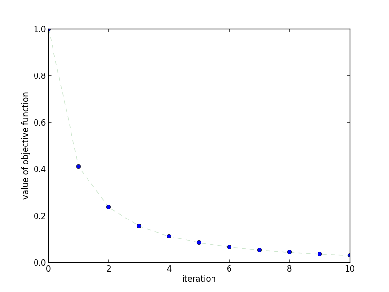This plot shows how quickly the objective function decreases as the number of iterations increases.

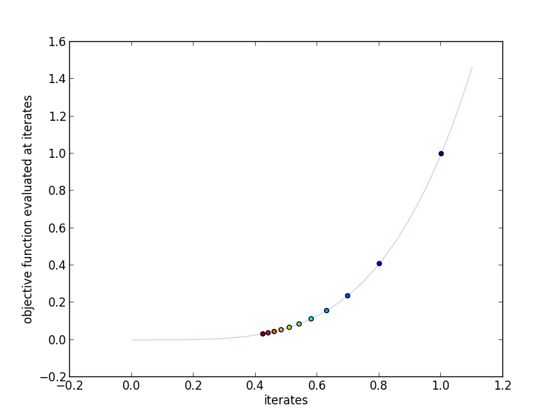This plot shows the actual iterates and the objective function evaluated at those points. More red indicates a higher iteration number.

Why does it work?

Gradient Descent works, but it isn't guaranteed to find the optimal solution to our problem (that is, \(x^{*} = \arg\min_{x} f(x)\)) without a few assumptions. In particular,

1. \(f\) is convex and finite for all \(x\)
2. a finite solution \(x^{*}\) exists
3. \(\nabla f(x)\) is Lipschitz continuous with constant \(L\). If \(f\) is twice differentiable, this means that the largest eigenvalue of the Hessian is bounded by \(L\) (\(\nabla^2 f(x) \preceq LI\)). But more directly, there must be an \(L\) such that,

Assumptions So what do these assumptions give us? Assumption 1 tells us that \(f\) is lower bounded by an affine function,

Assumption 3 also tells us that \(f\) is upper bounded by a quadratic (this is not obvious),

Proof Outline Now let's dive into the proof. Our plan of attack is as follows. First, we upper bound the error \(f(x^{(t+1)}) - f(x^{*})\) in terms of \(||x^{(t)} - x^{*}||_2^2\) and \(||x^{(t+1)} - x^{*}||_2^2\). We then sum these upper bounds across \(t\) to upper bound the sum of errors in terms of \(||x^{(0)} - x^{*}||_2^2\). Finally, we use the fact that \(f(x^{(t)})\) is decreasing in \(t\) to take an average of that sum to bound \(f(x^{(t+1)}) - f(x^{*})\) in terms of \(||x^{(0)} - x^{*}||_2^2\) and \(t\).

Step 1: upper bounding \(f(x^{(t+1)}) - f(x^{*})\). Let \(x^{+} \triangleq x^{(t+1)}\), \(x \triangleq x^{(t)}\), and \(\alpha \triangleq \alpha^{(t)}\).

Step 2: Upper bound \(\sum_{t=1}^{T} f(x^{(t)}) - f(x^{*})\) by summing across all \(t\). At this point we'll assume that \(\alpha^{(t)}\) is the same for all \(t\).

Step 3: Upper bound \(f(x^{(t+1)}) - f(x^{*})\) by using the fact that \(f(x^{(t+1)}) < f(x^{(t)})\)

Thus, we can conclude that if we want to reach an error tolerance \(f(x^{T}) - f(x^{*}) \le \epsilon\), we need \(O(\frac{1}{\epsilon})\) iterations. In other words, Gradient Descent has a "convergence rate" of \(O(\frac{1}{T})\).

When should I use it?

Because it's so easy to implement, Gradient Descent should be the first thing to try if you need to implement an optimization from scratch. So long as you calculate the gradient right, it's practically impossible to make a mistake. If you have access to an automatic differentiation library to do the gradient computation for you, even better! In addition, Gradient Descent requires a minimal memory footprint, making it ideal for problems where \(x\) is very high dimensional.

As we'll see in later posts, Gradient Descent trades memory for speed. The number of iterations required to reach a desired accuracy is actually quite large if you want accuracy on the order of \(10^{-8}\), and there are algorithms that are much faster if computation of the Hessian is feasible. Even when considering the same memory requirements, there is another gradient-based method with better convergence rates.

Extensions

Step Size The proof above relies on a constant step size, but quicker convergence can be obtained when using Line Search, wherein \(\alpha^{(t)}\) is chosen to (approximately) find \(\alpha^{(t)} = \arg\min_{\alpha} f(x^{(t)} - \alpha \nabla f(x^{(t)}))\). Keep in mind that unless \(0 \le t \le \frac{1}{L}\), Gradient Descent will not converge!

Checking Convergence We have shown that the algorithm's error at iteration \(T\) relies on \(T\) and the distance between \(x^{(0)}\) and \(x^{*}\), the latter of which is unknown. How then can we check if we're "close enough"? A typical choice is simply to stop after a fixed number of iterations, but another common alternative is to quit when \(||\nabla f(x^{(t)})||_2 < \epsilon_{g}\) for a chosen \(\epsilon_{g}\). The intuition for this comes from the assumption that \(f\) is "strongly convex" with constant \(m\), which then implies that \(||x - x^{*}||_2 \le \frac{2}{m}||\nabla f(x)||_2\) (see Convex Optimization, page 460, equation 9.10).

References

Proof of Convergence The proof of convergence for Gradient Descent is adapted from slide 1-18 of of UCLA's EE236C lecture on Gradient Methods.

Line Search The algorithm for Backtracking Line Search, a smart method for choosing step sizes, can be found on slide 10-6 of UCLA's EE236b lecture on unconstrained optimization.

Reference Implementation

Here's a quick implementation of gradient descent,

def gradient_descent(gradient, x0, alpha, n_iterations=100):
  """Gradient Descent

  Parameters
  ----------
  gradient : function
      Computes the gradient of the objective function at x
  x0 : array
      initial value for x
  alpha : function
      function computing step sizes
  n_iterations : int, optional
      number of iterations to perform

  Returns
  -------
  xs : list
      intermediate values for x
  """
  xs = [x0]
  for t in range(n_iterations):
    x = xs[-1]
    g = gradient(x)
    x_plus = x - alpha(t) * g
    xs.append(x_plus)
  return xs

# This generates the plots that appear above
if __name__ == '__main__':
  import os

  import numpy as np
  import pylab as pl
  import yannopt.plotting as plotting

  ### GRADIENT DESCENT ###

  # problem definition
  function = lambda x: x ** 4  # the function to minimize
  gradient = lambda x: 4 * x **3  # its gradient
  step_size = 0.05
  x0 = 1.0
  n_iterations = 10

  # run gradient descent
  iterates = gradient_descent(gradient, x0, lambda x: step_size, n_iterations=n_iterations)

  ### PLOTTING ###

  plotting.plot_iterates_vs_function(iterates, function,
                                     path='figures/iterates.png', y_star=0.0)
  plotting.plot_iteration_vs_function(iterates, function,
                                      path='figures/convergence.png', y_star=0.0)

  # make animation
  try:
    os.makedirs('figures/animation')
  except OSError:
    pass
  for t in range(n_iterations):
    x = iterates[t]
    x_plus = iterates[t+1]

    f = function
    g = gradient
    f_hat = lambda y: f(x) + g(x) * (y - x)

    x_min = (0-f(x))/g(x) + x
    x_max = (1.1-f(x))/g(x) + x

    pl.figure()

    pl.plot(np.linspace(0, 1.1, 100), function(np.linspace(0, 1.1, 100)), alpha=0.2)
    pl.xlim([0, 1.1])
    pl.ylim([0, 1.1])
    pl.xlabel('x')
    pl.ylabel('f(x)')

    pl.plot([x_min, x_max], [f_hat(x_min), f_hat(x_max)], '--', alpha=0.2)
    pl.scatter([x, x_plus], [f(x), f(x_plus)], c=[0.8, 0.2])

    pl.savefig('figures/animation/%02d.png' % t)
    pl.close()