In a previous post, I mentioned that one cannot hope to asymptotically outperform the $O(\frac{1}{\epsilon^2})$ convergence rate of Subgradient Descent when dealing with a non-differentiable objective function. This is in fact only half-true; Subgradient Descent cannot be beat using only first-order information (that is, gradients and subgradients). In this article, I'll describe Proximal Gradient Descent, an algorithm that exploits problem structure to obtain a rate of $O(\frac{1}{\epsilon})$. In particular, Proximal Gradient is useful if the following 2 assumptions hold. First, the objective function must be of the form,

$ \def\prox{\text{prox}} $

$$ \min_{x} \, g(x) + h(x) $$

with $g$ is differentiable. Second $h$ must be "simple" enough such that we can calculate its $\prox$ operator very quickly,

$$ \prox_{h}(x) = \min_{u} h(u) + \frac{1}{2} ||u-x||_2^2 $$

Using these two assumptions, we can obtain a convergence rate identical to Gradient Descent even when optimizing non-differentiable objective functions.

How does it work?

Input: initial iterate $x^{(0)}$

For $t = 0, 1, 2, \ldots$
1. Let $x^{(t+1)} = \prox_{ \alpha^{(t)} h } \left( x^{(t)} - \alpha^{(t)} \nabla g(x^{(t)}) \right)$
2. if converged, return $x^{(t+1)}$

Intuition for the $\prox$ Operator

At first sight, the $\prox$ operator looks suspicious. Where did it come from? Why did someone really think it would work? It ends up that we can derive the update for Gradient Descent and the update for Gradient Descent almost identically. First, notice that the Gradient Descent Update is the solution to the following quadratic approximation to $f(x)$.

$$ \begin{align*} x^{(t+1)} & = \arg\min_{y} f(x^{(t)}) + \nabla f(x^{(t)})^T (y-x^{(t)}) + \frac{L}{2} ||y-x^{(t)}||_2^2 \\ 0 & = \nabla f(x^{(t)}) + L (x^{(t+1)}-x^{(t)}) \\ x^{(t+1)} & = x^{(t)} - \frac{1}{L} \nabla f(x^{(t)}) \end{align*} $$

We take the gradient of the right hand side with respect to $y$ and set it to zero in the second line. Now replace $f$ with $g$, and add $h(y)$ to the very end of the first line,

$$ \begin{align*} x^{(t+1)} & = \arg\min_{y} g(x^{(t)}) + \nabla g(x^{(t)})^T (y-x^{(t)}) + \frac{L}{2} ||y-x^{(t)}||_2^2 + h(y) \\ & = \arg\min_{y} g(x^{(t)}) + \frac{L}{2} \left( \frac{2}{L} \nabla g(x^{(t)})^T (y-x^{(t)}) \right) + \frac{L}{2} ||y-x^{(t)}||_2^2 + h(y) + \frac{L}{2} ||\nabla g(x^{(t)})||_2^2 \\ & = \arg\min_{y} \frac{L}{2} || y - (x^{(t)} - \frac{1}{L} \nabla g(x^{(t)})) ||_2^2 + h(y) \\ & = \prox_{ \frac{1}{L} h }(x^{(t)} - \frac{1}{L} \nabla g(x^{(t)})) \\ \end{align*} $$

This time, we add constants (with respect to $y$) such that we can pull the $\nabla g(x^{(t)})^T (y-x^{(t)})$ into the quadratic term, leading us to the Proximal Gradient Descent update.

A Small Example

Let's now see how well Proximal Gradient Descent works. For this example, we'll solve the following problem,

$$ \min_{x} \, \log(1 + \exp(-2x)) + ||x||_1 $$

Letting $g(x) = \log(1+\exp(-2x))$ and $h(x) = ||x||_1$, it can be shown that,

$$ \begin{align*} \nabla g(x) &= \frac{1}{1 + \exp(-2x)} \left( \exp(-2x) \right) (-2) \\ \prox_{\alpha h}(x) & = \text{sign}(x) \max(0, \text{abs}(x) - \alpha) \\ \end{align*} $$

We'll use a variant of Backtracking Line Search modified for Proximal Gradient Descent and an initial choice of $x^{(0)} = 5$.

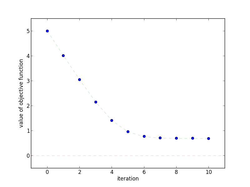
This plot shows how quickly the objective function decreases as the number of iterations increases.

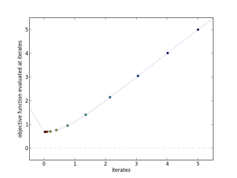
This plot shows the actual iterates and the objective function evaluated at those points. More red indicates a higher iteration number.

Why does it work?

Proximal Gradient Descent, like regular Gradient Descent, is a "descent" method where the objective value is guaranteed to decrease. In fact, the assumptions for Proximal Gradient Descent's $g(x)$ are the identical to the Gradient Descent assumptions for $f(x)$. The only additional condition is that $h(x)$ be convex,

$g(x)$ is convex, differentiable, and finite for all $x$
a finite solution $x^{*}$ exists
$\nabla g(x)$ is Lipschitz continuous with constant $L$. That is, there must be an $L$ such that,

$$ || \nabla g(x) - \nabla g(y) ||_2 \le L || x - y ||_2 \qquad \forall x,y $$

$h(x)$ is convex

Proof Outline The majority of the convergence proof for Proximal Gradient Descent is identical to the proof for regular Gradient Descent. The key is to carefully choose a function $G_{\alpha}(x)$ that can take the place of $\nabla f(x)$. Once it is defined, we can rephrase Proximal Gradient Descent as $x^{(t+1)} = x^{(t)} - \alpha^{(t)} G_{\alpha^{(t)}}(x^{(t)})$. Next, we'll show that,

$$ (g+h)(x^{(t+1)}) \le (g+h)(x^{*}) + G_{\alpha^{(t)}}(x^{(t)})^T (x-x^{*}) - \frac{\alpha^{(t)}}{2} ||G_{\alpha^{(t)}}(x^{(t)})||_2^2 $$

Once we have this, we can repeat the Gradient Descent proof verbatim with $g + h \rightarrow f$ and $G_{\alpha^{(t)}}(x^{(t)}) \rightarrow \nabla f(x^{(t)})$.

Step 1 Phrase Proximal Gradient Descent as $x^{(t+1)} = x^{(t)} - \alpha^{(t)} G_{\alpha^{(t)}}(x^{(t)})$. Define $G$ as follows,

$$ G_{\alpha}(x) \triangleq \frac{1}{\alpha} (x - \prox_{\alpha h}( x - \alpha \nabla g(x))) $$

Now let $x^{+} \triangleq x^{(t+1)}$, $x \triangleq x^{(t)}$, and $\alpha \triangleq \alpha^{(t)}$. Using $G$, we can reframe Proximal Gradient Descent as a typical descent method,

$$ \begin{align*} x^{+} &= x - \alpha G_{\alpha}(x) \\ &= x - \alpha \left( \frac{1}{\alpha} (x - \prox_{\alpha h}( x - \alpha \nabla g(x)) \right) \\ &= x - (x - \prox_{\alpha h}( x - \alpha \nabla g(x)) \\ &= \prox_{\alpha h}( x - \alpha \nabla g(x)) \\ \end{align*} $$

Step 2 Show that $G_{\alpha}(x)$ can be used like Gradient Descent's $\nabla f(x)$. Our goals is to obtain a statement identical to $f(x^{+}) \le f(x^{*}) + \nabla f(x)^T (x-x^{*}) - \frac{\alpha}{2} ||\nabla f(x)||_2^2$ except with $G_{\alpha}(x)$ instead of $\nabla f(x)$. Once we have this, the rest of the proof is exactly the same as Gradient Descent's. Begin by recalling the Lipschitz condition on $g$,

$$ g(y) \le g(x) + \nabla g(x)^T (y-x) + \frac{L}{2} ||y-x||_2^2 $$

Substitute $y = x^{+} = x - \alpha G_{\alpha}(x)$ to obtain,

$$ \begin{align*} g(x - \alpha G_{\alpha}(x)) & \le g(x) + \nabla g(x)^T(x - \alpha G_{\alpha}(x) - x) + \frac{L}{2}||x - \alpha G_{\alpha}(x) - x||_2^2 \\ & = g(x) - \alpha \nabla g(x)^T G_{\alpha}(x) + \frac{L ( \alpha )^2}{2}||G_{\alpha}(x)||_2^2 \\ \end{align*} $$

Assume then that $\alpha \le \frac{1}{L}$ (this is what Backtracking Line Search does), We can upper bound $\frac{L ( \alpha )^2}{2} \le \frac{\alpha}{2}$,

$$ \begin{align*} g(x - \alpha G_{\alpha}(x)) & \le g(x) - \alpha \nabla g(x)^T G_{\alpha}(x) + \frac{ \alpha }{2}||G_{\alpha}(x)||_2^2 \\ \end{align*} $$

Then add $h(x - \alpha G_{\alpha}(x))$ to both sides,

$$ \begin{align*} (g+h)(x - \alpha G_{\alpha}(x)) & \le g(x) - \alpha \nabla g(x)^T G_{\alpha}(x) + \frac{ \alpha }{2}||G_{\alpha}(x)||_2^2 \\ & \quad + h(x - \alpha G_{\alpha}(x)) \\ \end{align*} $$

Next, we'll upper bound $g(x)$ and $h(x - \alpha G_{\alpha}(x))$ using the definition of convexity. The following 2 equations hold for all $z$, For $g$, we'll use,

$$ \begin{align*} g(z) & \ge g(x) + \nabla g(x)^T (z-x) \\ g(z) + \nabla g(x)^T (x-z) & \ge g(x) \\ \end{align*} $$

For $h$ we have something a bit more mysterious,

$$ \begin{align*} h(z) & \ge h(x - \alpha G_{\alpha}(x)) + [G_{\alpha}(x) - \nabla g(x)]^T (z-(x - \alpha G_{\alpha}(x))) \\ h(z) + [G_{\alpha}(x) - \nabla g(x)]^T(x - \alpha G_{\alpha}(x) - z) & \ge h(x - \alpha G_{\alpha}(x)) \end{align*} $$

Where did that come from? It so happens that $G_{\alpha}(x) - \nabla g(x)$ is a valid subgradient for $h$ at $x - \alpha G_{\alpha}(x)$. Recall the 2 definitions we have for $x^{+}$,

$$ \begin{align*} x^{+} &= \prox_{\alpha h} (x - \alpha \nabla g(x)) \\ &= \arg\min_{u} \alpha h(u) + \frac{1}{2} ||u - (x - \alpha \nabla g(x))||_2^2 \\ 0 & \in \alpha \partial h(x^{+}) + x^{+} - (x - \alpha \nabla g(x)) \\ (x - \alpha \nabla g(x)) - x^{+} & \in \alpha \partial h(x^{+}) \\ (x - \alpha \nabla g(x)) - (x - \alpha G_{\alpha}(x)) & \in \alpha \partial h(x^{+}) \\ \alpha [G_{\alpha}(x)) - \nabla g(x)] & \in \alpha \partial h(x^{+}) \\ [G_{\alpha}(x)) - \nabla g(x)] & \in \partial h(x^{+}) \\ \end{align*} $$

Thus, $G_{\alpha}(x)) - \nabla g(x)$ is a valid subgradient for $h$ at $x^{+} \triangleq x - \alpha G_{\alpha}(x)$, and the previous lower bound on $h(z)$ holds. Putting the previous two inequalities back into the preceding equation and canceling out, we can see that for all $z$,

$$ \begin{align*} (g+h)(x - \alpha G_{\alpha}(x)) & \le g(x) - \alpha \nabla g(x)^T G_{\alpha}(x) + \frac{ \alpha }{2}||G_{\alpha}(x)||_2^2 \\ & \quad + h(x - \alpha G_{\alpha}(x)) \\ (g+h)(x - \alpha G_{\alpha}(x)) & \le \left( g(z) + \nabla g(z)^T (x-z) \right) - \alpha \nabla g(x)^T G_{\alpha}(x) + \frac{ \alpha }{2}||G_{\alpha}(x)||_2^2 \\ & \quad + \left( h(z) + [G_{\alpha}(x) - \nabla g(x)]^T (x - \alpha G_{\alpha}(x) - z) \right) \\ & = (g+h)(z) + G_{\alpha}(x)^T (x-z) - \frac{ \alpha }{2}||G_{\alpha}(x)||_2^2 \\ \end{align*} $$

Now let $z = x^{*}$ to get,

$$ \begin{align*} (g+h)(x^{+}) & \le (g+h)(x^{*}) + G_{\alpha}(x)^T (x-x^{*}) - \frac{ \alpha }{2}||G_{\alpha}(x)||_2^2 \\ \end{align*} $$

Looking back at Step 1 of the Gradient Descent Proof, you can see that this equation is exactly the same as the one used before except that $G_{\alpha}(x)$ replaces $\nabla f(x)$. Following the rest of the Gradient Descent proof, we find that of we want $(g+h)(x^{(t)}) - (g+h)(x^{*}) \le \epsilon$, we need $O(\frac{1}{\epsilon})$ iterations, just like Gradient Descent.

When should I use it?

Proximal Gradient Descent requires being able to easily calculate $\prox_{\alpha h}(x)$. The benefits of doing so are clear -- we can reach an $\epsilon$-approximate solution in far fewer iterations than Subgradient Descent. But this is only valuable if the cost of an iteration of Proximal Gradient Descent is similar to that of Subgradient Descent. For some choices of $h(x)$, this actually holds (see Common Prox Functions below); it is then that Proximal Gradient Descent should be used. For other cases where no closed-form solution exists, it is often better to stick with Subgradient Descent.

Extensions

Step Size The proof above assumes the step size $\alpha^{(t)} \le \frac{1}{L}$ ($L$ is the Lipschitz constant of $g(x)$). Rather than guessing for such values, Backtracking Line Search can be employed with a slight modification. Recall that Backtracking Line Search chooses $\alpha^{(t)}$ such that,

$$ \begin{align*} f(x^{(t)} - \alpha^{(t)} \nabla f(x^{(t)})) & \le f(x^{(t)}) - \frac{\alpha^{(t)}}{2}|| \nabla f(x^{(t)})||_2^2 \\ \end{align*} $$

If $\alpha^{(t)} \le \frac{1}{L}$, this statement must hold. To see why, let's write out where the condition came from,

$$ \begin{align*} f(x^{(t+1)}) & \le f(x^{(t)}) + \nabla f(^{(t)})^T (x^{(t+1)} - x^{(t)}) + \frac{1}{2 \alpha^{(t)}}||x^{(t+1)} - x^{(t)}||_2^2 \\ f(x^{(t)} - \alpha^{(t)} \nabla f(x^{(t)})) & \le f(x^{(t)}) + \nabla f(^{(t)})^T (x^{(t)} - \alpha^{(t)} \nabla f(x^{(t)}) - x^{(t)}) \\ & \quad + \frac{1}{2 \alpha^{(t)}}||x^{(t)} - \alpha^{(t)} \nabla f(x^{(t)}) - x^{(t)}||_2^2 \\ f(x^{(t)} - \alpha^{(t)} \nabla f(x^{(t)})) & \le f(x^{(t)}) - \alpha^{(t)} ||\nabla f(^{(t)}) ||_2^2 + \frac{\alpha^{(t)}}{2}|| \nabla f(x^{(t)})||_2^2 \\ f(x^{(t)} - \alpha^{(t)} \nabla f(x^{(t)})) & \le f(x^{(t)}) - \frac{\alpha^{(t)}}{2}|| \nabla f(x^{(t)})||_2^2 \\ \end{align*} $$

If we assume that $f$ is $L$-Lipschitz, then $\alpha^{(t)} = \frac{1}{L}$ is precisely the Lipschitz assumption. Recall now that for this problem, we have $G_{\alpha^{(t)}}(x^{(t)})$ in place of $\nabla f(x^{(t)})$. Replacing $f$ with $g+h$ and $\nabla f(x)$ with $G_{\alpha}(x)$, we come to a similar condition,

$$ \begin{align*} (g+h)(x^{(t+1)}) & \le (g+h)(x^{(t)}) - \frac{\alpha^{(t)}}{2}|| G_{\alpha^{(t)}}(x^{(t)}) ||_2^2 \\ \end{align*} $$

In other words, we can perform Backtracking Line Search for Proximal Gradient Descent as follows,

Input: iterate $x^{(t)}$, initial step size $\alpha_0$, step factor $\beta$

$\alpha = \alpha_0$
While True
1. Calculate $G_{\alpha}(x^{(t)}) = \frac{1}{\alpha}( x - \prox_{\alpha h}(x^{(t)} - \alpha \nabla g(x)) )$
2. if $(g+h)(x^{(t+1)}) \le (g+h)(x^{(t)}) - \frac{\alpha}{2}|| G_{\alpha}(x^{(t)}) ||_2^2$, set $\alpha^{(t)} = \alpha$ and return
3. otherwise set $\alpha \leftarrow \alpha \beta$ and continue

Common $\prox$ Functions

There are several common choices for $h(x)$ that admit particularly efficient $\prox$ functions. If your objective function contains one of these, consider applying Proximal Gradient immediately -- you'll converge far faster than Subgradient Descent.

$h(x)$	$\prox_{\alpha h}(x)$
$\|\|x\|\|_1$	$\text{sign}(x) \max(0, \text{abs}(x) - \alpha)$
$\frac{1}{2}\|\|x\|\|_2^2$	$\frac{1}{1 + \alpha} x$
$\|\|x\|\|_2$	$\left( 1 - \frac{\alpha}{\|\|x\|\|_2} \right) x$
$\|\|x\|\|_{\infty}$	$\text{sign}(x) \min( \text{abs}(x), \theta )$ where $\theta = \frac{1}{\rho} \sum_{j : \|x_j\| > \|x_{(\rho)}\|} (\|x_j\| - \alpha)$ where $x_{(i)}$ is is the $i$-th largest element of $x$ in magnitude and $\rho$ is the smallest $i$ such that $\sum_{j : \|x_j\| > \|x_{(i)}\|} (\|x_j\| - \|x_{(i)}\|) < \alpha$.
$\frac{1}{2} x^T Q x + b^T x$	$(\alpha Q + I)^{-1} (x - \alpha b)$

References

Proof of Convergence The original proof of convergence is thanks to Laurent El Ghaoui's EE227a slides.

List of Proximal FunctionsThe list of proximal functions is taken from John Duchi's article on Forward-Backward Splitting (FOBOS)

Reference Implementation

def proximal_gradient_descent(g_gradient, h_prox, x0,
                              alpha, n_iterations=100):
  """Proximal Gradient Descent

  Parameters
  ----------
  g_gradient : function
      Compute the gradient of `g(x)`
  h_prox : function
      Compute prox operator for h * alpha
  x0 : array
      initial value for x
  alpha : function
      function computing step sizes
  n_iterations : int, optional
      number of iterations to perform

  Returns
  -------
  xs : list
      intermediate values for x
  """
  xs = [x0]
  for t in range(n_iterations):
    x = xs[-1]
    g = g_gradient(x)
    step = alpha(x)
    x_plus = h_prox(x - step * g, step)
    xs.append(x_plus)
  return xs

def backtracking_line_search(g, h, g_gradient, h_prox):
  alpha_0 = 1.0
  beta    = 0.9
  def search(x):
    alpha = alpha_0
    while True:
      x_plus = h_prox(x - alpha * g_gradient(x), alpha)
      G = (1.0/alpha) * (x - x_plus)
      if g(x_plus) + h(x_plus) <= g(x) + h(x) - 0.5 * alpha * (G*G):
        return alpha
      else:
        alpha = alpha * beta
  return search


if __name__ == '__main__':
  import os

  import numpy as np
  import yannopt.plotting as plotting

  ### PROXIMAL GRADIENT DESCENT ###

  # problem definition
  g = lambda x: np.log(1 + np.exp(-2*x))
  h = lambda x: abs(x)
  function = lambda x: g(x) + h(x)
  g_gradient  = lambda x: -2 * np.exp(-x)/(1 + np.exp(-x))
  h_prox      = lambda x, alpha: np.sign(x) * max(0, abs(x) - alpha)
  alpha       = backtracking_line_search(g, h, g_gradient, h_prox)
  x0          = 5.0
  n_iterations = 10

  # run gradient descent
  iterates = proximal_gradient_descent(
                  g_gradient, h_prox, x0, alpha,
                  n_iterations=n_iterations
             )

  ### PLOTTING ###

  plotting.plot_iterates_vs_function(iterates, function,
                                     path='figures/iterates.png',
                                     y_star=0.69314718055994529)
  plotting.plot_iteration_vs_function(iterates, function,
                                      path='figures/convergence.png',
                                      y_star=0.69314718055994529)

Category: optimization
Tags: optimization , first-order , proximal

Strongly Convex

Proximal Gradient Descent