In this post, we'll take a look at the Frank-Wolfe Algorithm also known as the Conditional Gradient Method, an algorithm particularly suited for solving problems with compact domains. Like the Proximal Gradient and Accelerated Proximal Gradient algorithms, Frank-Wolfe requires we exploit problem structure to quickly solve a mini-optimization problem. Our reward for doing so is a converge rate of $O (1 / ϵ) <math xmlns="http://www.w3.org/1998/Math/MathML"><mi>O</mi><mo stretchy="false">(</mo><mn>1</mn><mrow data-mjx-texclass="ORD"><mo>/</mo></mrow><mi>ϵ</mi><mo stretchy="false">)</mo></math>$ and the potential for extremely sparse solutions.

Returning to my valley-finding metaphor, Frank-Wolfe is a bit like this,

Look around you and see which way points the most downwards
Walk as far as possible in that direction until you hit a wall
Go back in the direction you started, stop part way along the path, then repeat.

How does it work?

Frank-Wolfe is designed to solve problems of the form,

min <math xmlns="http://www.w3.org/1998/Math/MathML" display="block"><munder><mo data-mjx-texclass="OP" movablelimits="true">min</mo><mrow data-mjx-texclass="ORD"><mi>x</mi><mo>\in</mo><mi>D</mi></mrow></munder><mi>f</mi><mo stretchy="false">(</mo><mi>x</mi><mo stretchy="false">)</mo></math>

where $D$ is compact and $f$ is differentiable. For example, in $R^{n}$ any closed and bounded set is compact. The algorithm for Frank-Wolfe is then,

Input: Initial iterate $x^{(0)}$

For $t = 0, 1, 2, \dots$
1. Let $s^{(t + 1)} = \arg min_{s \in D} ⟨ \nabla f (x^{(t)}), s ⟩$
2. If $g (x) = ⟨ \nabla f (x^{(t)}), x - s^{(t + 1)} ⟩ \leq ϵ$ , break
3. Let $x^{(t + 1)} = (1 - α^{(t)}) x^{(t)} + α^{(t)} s^{(t + 1)}$

The proof relies on $α^{(t)} = 2 / (t + 2)$ , but line search works as well. The intuition for the algorithm is that at each iteration, we minimize a linear approximation to $f$ ,

s^{(t + 1)} = \arg min_{s \in D} f (x^{(t)}) + \nabla f (x^{(t)})^{T} (s - x^{(t)})

then take a step in that direction. We can immediately see that if $D$ weren't compact, $s^{(t)}$ would go off to infinity.

Upper Bound One nice property of Frank-Wolfe is that it comes with its own upper bound on $f (x^{(t)}) - f (x^{*})$ calculated during the course of the algorithm. Recall the linear upper bound on $f$ due to convexity,

\begin{aligned} f (x^{*}) & \geq f (x) + \nabla f (x)^{T} (x^{*} - x) \\ f (x) - f (x^{*}) & \leq \nabla f (x)^{T} (x - x^{*}) \end{aligned}

Since,

s^{(t + 1)} = \arg min_{s} \nabla f (x^{(t)})^{T} s = \arg max_{s} \nabla f (x^{(t)})^{T} (x^{(t)} - s)

we know that $\nabla f (x^{(t)})^{T} (x^{(t)} - x^{*}) \leq \nabla f (x^{(t)})^{T} (x^{(t)} - s^{(t + 1)})$ and thus,

f (x) - f (x^{*}) \leq \nabla f (x^{(t)})^{T} (x^{(t)} - s^{(t + 1)})

A Small Example

For this example, we'll minimize a simple univariate quadratic function constrained to lie in an interval,

min_{x \in [- 1, 2]} (x - 0.5)^{2} + 2 x

Its derivative is given by $2 (x - 0.5) + 2$ , and since we are dealing with real numbers, the minimizers of the linear approximation must be either $- 1$ or $2$ if the gradient is positive or negative, respectively. We'll use a stepsize of $α^{(t)} = 2 / (t + 2)$ as prescribed by the convergence proof in the next section.

Frank-Wolfe in action. The red circle is the current value for $f(x^{(t)})$, and the green diamond is $f(x^{(t+1)})$. The dotted line is the linear approximation to $f$ at $x^{(t)}$. Notice that at each step, Frank-Wolfe stays closer and closer to $x^{(t)}$ when moving in the direction of $s^{(t+1)}$.

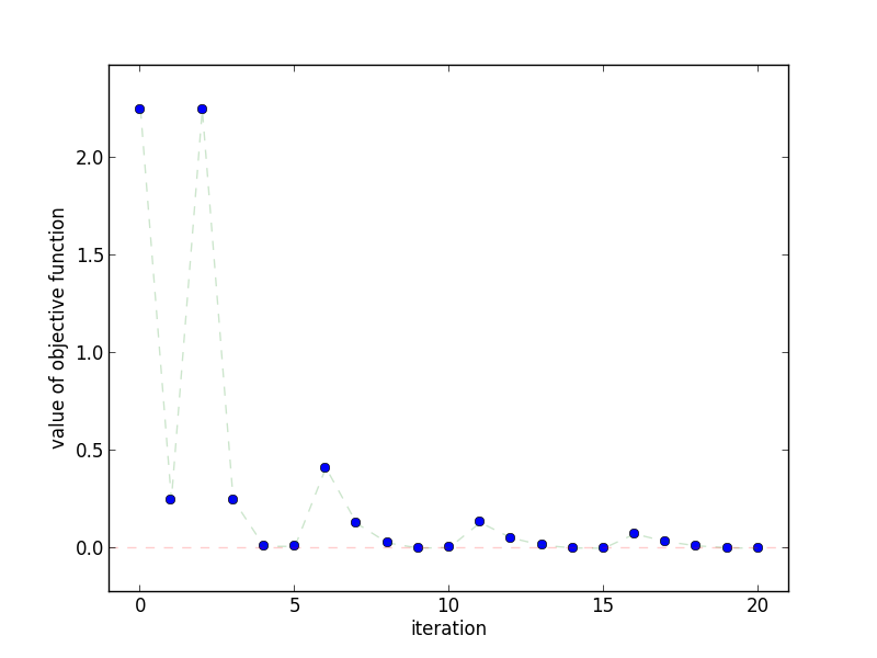This plot shows how quickly the objective function decreases as the number of iterations increases. Notice that it does not monotonically decrease, as with Gradient Descent.

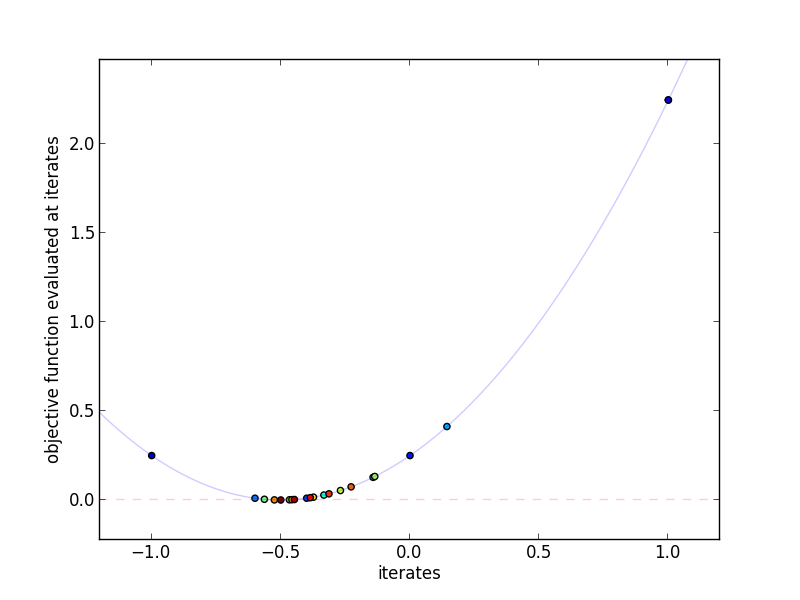This plot shows the actual iterates and the objective function evaluated at those points. More red indicates a higher iteration number. Since Frank-Wolfe uses linear combinations of $s^{(t+1)}$ and $x^{(t)}$, it tends to "bounce around" a lot, especially in earlier iterations.

Why does it work?

We begin by making the two assumptions given earlier,

$f$ is convex, differentiable, and finite for all $x \in D$
$D$ is compact

Assumptions First, notice that we never needed to assume that a solution $x^{*}$ exists. This is because $D$ is compact and $f$ is finite, meaning $x$ cannot get bigger and bigger to make $f (x)$ arbitrarily small.

Secondly, we never made a Lipschitz assumption on $f$ or its gradient. Since $D$ is compact, we don't have to -- instead, we get the following for free. Define $C_{f}$ as,

C_{f} = max_{\begin{matrix} x, s \in D \\ α \in [0, 1] \\ y = x + α (s - x) \end{matrix}} \frac{2}{α^{2}} (f (y) - f (x) - ⟨ \nabla f (x), y - x ⟩)

This immediate implies the following upper bound on $f$ for all $x, y \in D$ and $α \in [0, 1]$ ,

f (y) \leq f (x) + ⟨ \nabla f (x), y - x ⟩ + \frac{α^{2}}{2} C_{f}

Proof Outline The proof for Frank-Wolfe is surprisingly simple. The idea is to first upper bound $f (x^{(t + 1)})$ in terms of $f (x^{(t)})$ , $g (x^{(t)})$ , and $C_{f}$ . We then transform this per-iteration bound into a bound on $f (x^{(t)}) - f (x^{*})$ depending on $t$ using induction. That's it!

Step 1 Upper bound $f (x^{(t + 1)})$ . As usual, we'll denote $x^{+} ≜ x^{(t + 1)}$ , $x ≜ x^{(t)}$ , $s^{+} ≜ s^{(t + 1)}$ , and $α ≜ α^{(t)}$ . We begin by using the upper bound we just obtained for $f$ in terms of $C_{f}$ , substituting $x^{+} = (1 - α) x + α s^{+}$ and then $g (x) = \nabla f (x)^{T} (x - s^{+})$ ,

\begin{aligned} f (x^{+}) & \leq f (x) + \nabla f (x)^{T} (x^{+} - x) + \frac{α^{2}}{2} C_{f} \\ = f (x) + \nabla f (x)^{T} ((1 - α) x + α s^{+} - x) + \frac{α^{2}}{2} C_{f} \\ = f (x) + \nabla f (x)^{T} (α s^{+} - α x) + \frac{α^{2}}{2} C_{f} \\ = f (x) - α \nabla f (x)^{T} (x - s^{+}) + \frac{α^{2}}{2} C_{f} \\ = f (x) - α g (x) + \frac{α^{2}}{2} C_{f} \end{aligned}

Step 2 Use induction on $t$ . First, recall the upper bound on $f (x) - f (x^{*}) \leq g (x)$ we derived above. Let's add $- f (x^{*})$ into what we got from Step 1, then use the upper bound on $f (x) - f (x^{*})$ to get,

\begin{aligned} f (x^{+}) - f (x^{*}) & \leq f (x) - f (x^{*}) - α g (x) + \frac{α^{2}}{2} C_{f} \\ \leq f (x) - f (x^{*}) - α (f (x) - f (x^{*})) + \frac{α^{2}}{2} C_{f} \\ = (1 - α) (f (x) - f (x^{*})) + \frac{α^{2}}{2} C_{f} \end{aligned}

Now, we employ induction on $t$ to show that,

f (x^{(t)}) - f (x^{*}) \leq \frac{4 C_{f} / 2}{t + 2}

We'll assume that the step size is $α^{(t)} = \frac{2}{t + 2}$ , giving us $α^{(0)} = 2 / (0 + 2) = 1$ and the base case,

\begin{aligned} f (x^{(1)} - f (x^{*}) & \leq (1 - α^{(0)}) (f (x^{(0)}) - f (x^{*})) + \frac{α^{2}}{2} C_{f} \\ = (1 - 1) (f (x^{(0)}) - f (x^{*})) + \frac{1}{2} C_{f} \\ \leq \frac{4 C_{f} / 2}{(0 + 1) + 2} \end{aligned}

Next, for the recursive case, we use the inductive assumption on $f (x) - f (x^{*})$ , the definition of $α^{(t)}$ , and some algebra,

\begin{aligned} f (x^{+}) - f (x^{*}) & \leq (1 - α) (f (x) - f (x^{*})) + \frac{α^{2}}{2} C_{f} \\ \leq (1 - \frac{2}{t + 2}) \frac{4 C_{f} / 2}{t + 2} + {(\frac{2}{t + 2})}^{2} C_{f} / 2 \\ \leq \frac{4 C_{f} / 2}{t + 2} (1 - \frac{2}{t + 2} + \frac{1}{t + 2}) \\ = \frac{4 C_{f} / 2}{t + 2} (\frac{t + 1}{t + 2}) \\ \leq \frac{4 C_{f} / 2}{t + 2} (\frac{t + 2}{t + 3}) \\ = \frac{4 C_{f} / 2}{(t + 1) + 2} \end{aligned}

Thus, if we want an error tolerance of $ϵ$ , we need $O (\frac{1}{ϵ})$ iterations to find it. This matches the convergence rate of Gradient Descent an Proximal Gradient Descent, but falls short of their accelerated brethren.

When should I use it?

Like Proximal Gradient, efficient use of Frank-Wolfe requires solving a mini-optimization problem at each iteration. Unlike Proximal Gradient, however, this mini-problem will lead to unbounded iterates if the input space is not compact -- in other words, Frank-Wolfe cannot directly be applied when your domain is all of $R^{n}$ . However, there is a very special case wherein Frank-Wolfe shines.

Sparsity The primary reason machine learning researchers have recently taken an interest in Frank-Wolfe is because in certain problems the iterates $x^{(t)}$ will be extremely sparse. Suppose that $D$ is a polyhedron defined by a set of linear constraints. Then $s^{(t)}$ is a solution to a Linear Program, meaning that each $s^{(t)}$ lies on one of the vertices of the polyhedron. If these vertices have only a few non-zero entries, then $x^{(t)}$ will too, as $x^{(t)}$ is a linear combination of $s^{(1)} \dots s^{(t)}$ . This is in direct contrast to gradient and proximal based methods, wherein $x^{(t)}$ is the linear combination of a set of non-sparse gradients.

| | x | | = inf {t : x \in t Conv (A)}

For example, $| | x | |_{1}$ is an atomic norm with $A$ being the set of all vectors with only one $+ 1$ or one $- 1$ entry. In these cases, finding $\arg min_{| | s | | \leq c} ⟨ \nabla f (x), s ⟩$ is tantamount to finding which element of $A$ minimizes $⟨ \nabla f (x), s ⟩$ (since $Conv (A)$ defines a polyhedron). For a whole lot more on Atomic Norms, see this tome by Chandrasekaranm et al.

Extensions

Step Size The proof above relied on a step size of $α^{(t)} = \frac{2}{t + 2}$ , but as usual Line Search can be applied to accelerate convergence.

Approximate Linear Solutions Though not stated in the proof above, another cool point about Frank-Wolfe is that you don't actually need to solve the linear mini-problem exactly, but you will still converge to the optimal solution (albet at a slightly slower rate). In particular, assume that each mini-problem can be solved approximately with additive error $\frac{δ C_{f}}{t + 2}$ at iteration $t$ ,

⟨ s^{(t + 1)}, \nabla f (x^{(t)}) ⟩ \leq min_{s} ⟨ s, \nabla f (x^{(t)}) ⟩ + \frac{δ C_{f}}{t + 2}

then Frank-Wolfe's rate of convergence is

f (x^{(t)}) - f (x^{*}) \leq \frac{2 C_{f}}{t + 2} (1 + δ)

The proof for this can be found in the supplement to Jaggi's excellent survey on Frank-Wolfe for machine learning.

Linear Invariance

Another cool fact about Frank-Wolfe is that it's linearly invariant -- that is, if you rotate and scale the space, nothing changes about the convergence rate. This is in direct contrast to many other methods which depend on the condition number of a function (for functions with Hessians, this is the ratio between the largest and smallest eigenvalues, $σ_{max} / σ_{min})$ .

Suppose we transform our input space with a surjective (that is, onto) linear transformation $M : \hat{D} \to D$ . Let's now try to solve the problem,

min_{\hat{x} \in \hat{D}} \hat{f} (\hat{x}) = f (M \hat{x}) = f (x)

Let's look at the solution to the per-iteration mini-problem we need to solve for Frank-Wolfe,

\begin{array}{r} min_{\hat{s} \in \hat{D}} ⟨ \nabla \hat{f} (\hat{x}), \hat{s} ⟩ = min_{\hat{s} \in \hat{D}} ⟨ M^{T} \nabla f (M \hat{x}), \hat{s} ⟩ = min_{\hat{s} \in \hat{D}} ⟨ \nabla f (x), M \hat{s} ⟩ = min_{s \in D} ⟨ \nabla f (x), s ⟩ \end{array}

In other words, we will find the same $s$ if we solve in the original space, or if we find $\hat{s}$ and then map it back to $s$ . No matter how $M$ warps the space, Frank-Wolfe will do the same thing. This also means that if there's a linear transformation you can do to make the points of your polyhedron sparse, you can do it with no penalty!

References

Proof of Convergence, Linear Invariance Pretty much everything in this article comes from Jaggi's fantastic article on Frank-Wolfe for machine learning.

Reference Implementation

def frank_wolfe(minisolver, gradient, alpha, x0, epsilon=1e-2):
  """Frank-Wolfe Algorithm

  Parameters
  ----------
  minisolver : function
      minisolver(x) = argmin_{s \in D} <x, s>
  gradient : function
      gradient(x) = gradient[f](x)
  alpha : function
      learning rate
  x0 : array
      initial value for x
  epsilon : float
      desired accuracy
  """
  xs = [x0]
  iteration = 0
  while True:
    x = xs[-1]
    g = gradient(x)
    s_next = minisolver(g)
    if g * (x - s_next) <= epsilon:
      break
    a = alpha(iteration=iteration, x=x, direction=s_next)
    x_next = (1 - a) * x + a * s_next
    xs.append(x_next)
    iteration += 1
  return xs


def default_learning_rate(iteration, **kwargs):
  return 2.0 / (iteration + 2.0)


if __name__ == '__main__':
  import os

  import numpy as np
  import pylab as pl
  import yannopt.plotting as plotting

  ### FRANK WOLFE ALGORITHM ###

  # problem definition
  function    = lambda x: (x - 0.5) ** 2 + 2 * x
  gradient    = lambda x: 2 * (x - 0.5) + 2
  minisolver  = lambda y: -1 if y > 0 else 2 # D = [-1, 2]
  x0 = 1.0

  # run gradient descent
  iterates = frank_wolfe(minisolver, gradient, default_learning_rate, x0)

  ### PLOTTING ###

  plotting.plot_iterates_vs_function(iterates, function,
                                     path='figures/iterates.png', y_star=0.0)
  plotting.plot_iteration_vs_function(iterates, function,
                                      path='figures/convergence.png', y_star=0.0)

  # make animation
  iterates = np.asarray(iterates)
  try:
    os.makedirs('figures/animation')
  except OSError:
    pass

  for t in range(len(iterates)-1):
    x = iterates[t]
    x_plus = iterates[t+1]
    s_plus = minisolver(gradient(x))

    f = function
    g = gradient
    f_hat = lambda y: f(x) + g(x) * (y - x)

    xmin, xmax = plotting.limits([-1, 2])
    ymin, ymax = -4, 8

    pl.plot(np.linspace(xmin ,xmax), function(np.linspace(xmin, xmax)), alpha=0.2)
    pl.xlim([xmin, xmax])
    pl.ylim([ymin, ymax])
    pl.xlabel('x')
    pl.ylabel('f(x)')

    pl.plot([xmin, xmax], [f_hat(xmin), f_hat(xmax)], '--', alpha=0.2)
    pl.vlines([-1, 2], ymin, ymax, color=np.ones((2,3)) * 0.2, linestyle='solid')
    pl.scatter(x, f(x), c=[0.8, 0.0, 0.0], marker='o', alpha=0.8)
    pl.scatter(x_plus, f(x_plus), c=[0.0, 0.8, 0.0], marker='D', alpha=0.8)
    pl.vlines(x_plus, f_hat(x_plus), f(x_plus), color=[0.0,0.8,0.0], linestyle='dotted')
    pl.scatter(s_plus, f_hat(s_plus), c=0.35, marker='x', alpha=0.8)

    pl.savefig('figures/animation/%02d.png' % t)
    pl.close()

Category: optimization
Tags: optimization , first-order , sparsity